 Decision making is the process that leads to a choice between a set of alternatives. Geographical decision-making means analysing and interpreting geographical information that is related to the alternatives in question. Decision making is often used in land suitability analysis, or site selection, as well as location allocation modelling. This paper below was written by Jan Husdal in 1999 as part of his coursework for the MSc in GIS at the University of Leicester, UK. Later revised in 2002 and 2008, it will address some of the aspects of decision making and describe some of approaches used.
Uncertainty
All decision making has a degree of uncertainty, ranging from a predictable (deterministic) situation to an uncertain situation (Malczewski, 1999). The latter one can be subdivided into stochastic decisions (which can be modelled by probability theory and statistics) and fuzzy decisions (which can modelled by fuzzy set theory and others). Consequently, particularly in uncertain situations, decision making involves the risk of making a “wrong” decision, because the information acquired is insufficient or the approach used is inappropriate. When uncertainty is part of the process, this uncertainty may in some cases be quantified and as such add another decision criteria to the evaluation process.
Objectives versus criteria
Most geographical decisions can de described in one of the following 3 categories (Fisher, 1999):
Single objective – Single criteria
Single objective – Multi criteria
Multi objective – Multi criteria
An objective is the ultimate goal that is to be achieved, i.e. finding the 5000 ha of land best suited for residential development. A criterion is a concrete descriptive variable from which the objective is inferred from, i.e. soil type, slope, proximity to roads, or development cost. In dealing with multiple criteria, the first obstacle in decision making is finding comprehensive criteria. The second obstacle is determining which criteria are more important than others and how to weight them.
Constraints versus factors
A constraint is a criterion that is absolute in its inclusion or exclusion of possible outcomes. This might be a boundary for a development area, slopes that are too steep or other attributes. A factor is a criterion that influences the suitability of the decision, according to its value. Different factors might be assigned with different weighting to illustrate their individual importance.
The decision making process
Decision making is a sequential process (based on Malczewski, 1999):
- Defining the decision problem (objective)
- Determining the set of evaluation criteria to be used
- Weighting the criteria Generating alternatives
- Applying decision rules
- Recommending the best solution to the problem
Any decision-making process begins with the definition of the problem or the objective to be reached. Once the decision problem is defined, what follows is setting up a set of criteria that reflect all concerns of the problem and finding measures as to which the degree is achieved.
The purpose of weights is to express the importance or preference of each criterion relative to other criteria. Alternatives are often determined by constraints, which limit the decision space of feasible alternatives. Decision rules integrate criteria, weights and preferences to generate an overall assessment of the alternatives. Recommendations are based on a ranking of the alternatives, with reference to possible uncertainties or sensitivities. Sensitivities are changes in the input of the analysis that bias the outcome.
Weighting
Multiple criteria typically have varying importance. To illustrate this, each criterion can be assigned a specific weight that reflects it importance relative to other criteria under consideration. The weight value is not only dependent the importance of any criterion, it is also dependent on the possible range of the criterion values. A criterion with variability will contribute more to the outcome of the alternative and should consequently be regarded as more important than criteria with no or little changes in their range.
Weights are usually normalised to sum up to 1, so that in a set of weights (w1, w2, ., wn) =1.
There are several methods for deriving weights, among them (Malczewski, 1999):
- Ranking
- Rating
- Pairwise Comparison
- Trade-off
The simplest way is straight ranking (in order of preference: 1=most important, 2=second most important, etc.). Then the ranking is converted into numerical weights on a scale from 0 to 1, so that they sum up to 1.
IDRISI features a weight routine to calculate weights, based on the pairwise comparison method, developed by Saaty (1980). A matrix is constructed, where each criterion is compared with the other criteria, relative to its importance, on a scale from 1 to 9. Then, a weight estimate is calculated and used to derive a consistency ratio (CR) of the pairwise comparisons, If CR > 0.10, then some pairwise values need to be reconsidered and the process is repeated till the desired value of CR < 0.10 is reached.
Multi-criteria / single objective decision making
The most used analytical facilities in a GIS is overlaying several thematic layers to find areas that are common to given criteria, or areas that exclude each other. In finding the solution to achieve one objective this is often done by sieve mapping, sifting through the layers to find location that encompass all desired criteria.
Boolean constraints
The easiest way to do sieve mapping to use Boolean logic to find combinations of layers that are defined by using logical operators: AND for intersection, OR for union, and NOT for exclusion of areas (Jones, 1997). In this approach, the criterion is either true or false. Areas are designated by a simple binary number, 1, including, or 0, excluding them from being suitable for consideration (Eastman, 1999).
Boolean operators
Each criteria is of equal value

Within 500m from Shepshed

Within 450m from roads

Slope between 0 and 2.5%

Land grade III

Suitable land, min 2.5 ha
Fuzzy variables
This approach attempts to turn the artificially crisp and clear-cut criteria of the simple Boolean approach into real-life continuous criteria that express a degree of suitability. Criteria can be modelled as a continuous variable ranging from most suitable (value 1) to least suitable (value 0).
Fuzzy approach
Bright areas have highest suitability

100m < Shepshed <1000m

Between 50m and
600m to roads

Slope between 1 and 5%

Land grade III and grade IV

Varying suitability,
min 2.5 ha
Comparison of different approaches
Boolean constraints

The Boolean constrains leave no room for prioritisation, all suitable areas are of equal value, regardless of their position in reference to their factors.
Minimal membership

In the minimal fuzzy membership the minimum suitability value from each factor at that location is chosen from as the “worst case” suitability. This results in larger areas, with highly suitable areas, with area that are more suitable shown in a brighter colour.
Probabilistic intersection

The probabilistic fuzzy intersection has less suitable areas than the minimal fuzzy operation. This is due to the fact that this effectively is a multiplication. Multiplying suitability factors of 0.9 and 0.9 at one location yields an overall suitability of 0.81, whereas the fuzzy approach results in 0.9. Thus, it can be argued that the probabilistic operation is counterproductive when using fuzzy variables (Fisher, 1994). When using suitability values larger than 1 this does of course not occur.
Weighted Overlay

The weighted overlay produces many more areas. This shows all possible solutions, regardless whether all factors apply or not, as long as at least one factor is valid for that area. This is so, because even if one factor is null, the other factors still sum up to a value. This also shows areas that are outside of the initial constraints.
Multi-criteria / Multi-objective decision making
The multi-objective decision making process is similar to single objective. One added aspect is that objectives can be complementing, but more often they are conflicting, and a compromising solution must be sought.
Simple Additive Weighting
Simple Additive Weighting (SAW) or Weighted Linear Combination (WLC) is the most often used technique in multi-criteria decision making. Criteria here may include weighted factors and constraints.
Calculating the product of weight and factor multiplied with all constraints at any location, and then summing up all products yields a total overall score. The score for each alternative A is:
A = SUM (wi * xi) or A = SUM (wi * xi) * SUM (cj)
if a constraint is part of the decision
xi = criterion score of factor i,
wi = weight of factor i,
cj = criterion score of constraint j
When applying SAW on fuzzy variables the formula can be applied directly, because the values all are in range from 0 to 1and directly comparable. In other cases the values for each criterion range must be standardised on the same scale. This is achieved by stretching the values so that they meet the same scale. If the continuous scale ranges from 0 to 255, a location with value of 123 in proximity to road and a location with a value of 123 in slope gradient means that the two locations initially, before SAW is applied, are equally suitable with respect to their criteria. This is why factor maps need to be stretched before they can be used in the MCE module.
WLC, single objective:
Best 1000 ha for industrial development
Standardised factors (constraints not shown):

Proximity to roads

Proximity to town

Slopes

Distance from park
Suitability maps:

SAW, result:
Area suited for industry

Ranking yields:
Best 1000 ha for industry
The above shows an ordinary weighted linear combination for a single objective. The image series below demonstrates that when multiple objectives must be met, the suitability for each objective can be used as factor for the multi-objective task.
WLC, Complementary objectives:
Best 4000 ha for both industrial and residential development
Standardised factors:
(constraints not shown)

Suitability for industrial development, standardised from suitability for industry above

Suitability for residential development, standardised from suitability for residential development, derived in similar manner as industrial suitability above.
Suitability maps:

SAW: Suitability for urban and residential development

Best 4000 ha for urbanisation
When objectives are conflicting, the higher priority is solved first, and then used as a mask for the lower priority in its calculation. Thus, there will be no overlapping, but zoning of allocations.
Conflicting objectives
Protecting 6000 ha of agriculture from urbanization,
Urbanisation has priority over agriculture
Standardised factors
(constraints not shown):

Proximity to roads

Proximity to town

Slopes

Distance from park

Rainfall
Suitability maps:

Suitable for urbanisation, derived from above

Suitable for agriculture

Suitable for agriculture, with the best 4000 ha for urbanisation masked out

Best 6000 ha for agriculture, with priority to 4000 ha for urbanisation

Final allocation of land for urbanisation and agriculture
Multi Objective Land Allocation
Multi Objective Land Allocation (MOLA) provides a procedure for solving multi-objective land allocation problems for cases with conflicting objectives. It determines a compromise solution that attempts to maximize the suitability of lands for each objective with respect to their assigned weights. In practical terms, after each objective has been given its suitability, MOLA will allocate areas from each objective according to their ranking and weighting, using an iterative process.
Making a pairwise comparison, MOLA resolves any conflict by allocating each cell to the objective to which its total weighted suitability is nearest. As a result, any particular objective will lose some conflict cases because it will need to accept cells that are of lower rank for itself, but of higher rank for any other objective (Jones, 1997).
MOLA, Conflicting objectives:
Protecting 6000 ha of agricultural land
while leaving 1500 ha for industrial development
Step 1
Standardised factors:

Proximity to water

Proximity to power

Proximity to roads

Proximity to market

Slope
Step 2
Suitability for each objective:

Agriculture

Carpet industry

Best 6000 ha for agriculture

Best 1500 ha for carpet industry

Conflict area
Step 3
MOLA

Compromise solution
It can be noted that industry is located particularly close to where roads and rivers coincide. This is consistent with the fact that proximity to water and power respectively has the highest weighting for agricultural development and industrial location respectively, since power lines were assumed to be along major roads.
Discussion
In the Boolean Intersection all criteria are assumed to be constraints. Suitability in one constraint will not compensate for non-suitability in any other constraint. This procedure also seems to carry the lowest possible uncertainty since only areas considered suitable in all criteria are entered into the result. However, this method requires crisp entities as criteria, a requirement that may be hard to meet. The advantage of the Boolean Intersection is that is straightforward and easy to apply. A disadvantage is that it might exclude or include areas that are not truly represented. Boolean Intersection is best applied either as a crude estimation or when all factors are of equal weight and when it can be assumed that the factors are of equal importance in any of the area they cover.
Weighted Linear Combination allows each factor to display its potential because of the factor weights. Factor weights are very important in WLC because they determine how individual factors will aggregate. Thus, deciding on the correct weighting becomes essential. The advantage of this method is that all factors contribute to the solution based on their importance. The aggregation of individual weights is prone to be very subjective, even when pairwise comparison is used for ensuring consistent weights.
Multi Objective Land Allocation blends priorities, whereas WLC favors one over the other, creating zones that do not overlap. MOLA is therefore preferable for solving conflicts that arise when multiple objectives whish to acquire the same area and where an incorrect decision might be highly damaging.
Conclusion
A GIS has the capacity to integrate information form a variety of sources into a spatial context and is well suited to support decision making procedures. GIS can act as a tool in helping the decision-makers evaluate alternatives, visualise choices and explore certain alternatives.
In the end, it is the decision maker, who determines the criteria, the factors, the constraints, the individual weighting and the decision rules.
There is also a multitude of other approaches to decision making not mentioned in this essay. Consequently, there is great room for bias in the decision making process.
References
Eastman, J.R. (1999) Multi-criteria evaluation and GIS
Longley, Goodchild, Maguire and Rhind (Eds.) Geographical Information Systems: Principles, Techniques, Applications and Management, 2nd Edition, Vol. 1, pp 493 -502
Fisher, P.F. (1994) Probable and fuzzy models of the viewshed operation. Innovations in GIS 1, pp. 161-175
Fisher, P.F. (1999) GY 705 Geographical Decision Making, University of Leicester, Lecture notes and practical tutorials
Jones, C. (1997) Geographical Information Systems and Computer Cartography, pp. 215 – 230
Malczewski, J. (1999) GIS and Multicriteria Decision Analysis